library(tidyverse)
library(readxl)
library(janitor)
library(countrycode)
library(paletteer)

theme_base <-
    theme(
    plot.margin = margin(10,5,5,5),
    axis.ticks = element_line(),
    axis.line.y = element_line(),
    legend.position = "top",
    legend.box = "vertical"
  )

a <- theme_set(
  theme_minimal(
    base_size = 12,
  ) +
    theme_base
)Unbalanced Rejection Rates of Schengen Short Stay Visas
Background

This is an extract of an analysis done by Marta Foresti and me as part of the activity of the LAGO Collective on how unfair and strict Schengen short stay visa policies might be hurting the development of the EU states, instead of protecting them.
This is a very short exploration of the same data done for teaching purposes.
Introduction
The Schengen area grants short stay visas for visitors staying no longer than 90 days. And releases detailed statistics on the acceptance rate by consulate in which the request was lodged. Can we detect hint of an unbalance in those data?
Analysis
Packages and Setup
Data
2022 statistics are available at the website for Home Affairs of the European Commission in excel format.
I’ve downloaded them manually and added them into the data folder.
Let’s read and clean them:
data_path <- 'data/Visa statistics for consulates in 2022_en.xlsx'

visa <-
  read_excel(
    data_path,
    sheet = 2
  ) %>%
  clean_names() %>%
  select(
    schengen_state,
    consulate_country = country_where_consulate_is_located,
    consulate_city = consulate,
    issued = total_at_vs_and_uniform_visas_issued_including_multiple_at_vs_me_vs_and_lt_vs,
    not_issued = total_at_vs_and_uniform_visas_not_issued
  )
The visa dataset now looks like this:
visa %>% glimpse()Rows: 1,773
Columns: 5
$ schengen_state <chr> "Austria", "Austria", "Austria", "Austria", "Austria…
$ consulate_country <chr> "ALBANIA", "ALGERIA", "ARGENTINA", "AUSTRALIA", "AZE…
$ consulate_city <chr> "TIRANA", "ALGIERS", "BUENOS AIRES", "CANBERRA", "BA…
$ issued <dbl> 81, 1216, 18, 1754, 1755, 1530, 50, 378, 643, 21, 81…
$ not_issued <dbl> 6, 831, NA, 22, 33, 13, NA, 4, 8, NA, 310, 17, NA, 8…Missing Data
visa %>%
  summarise(
    across(
      .cols = everything(),
      .fns = ~is.na(.) %>% sum()
    )
  ) %>%
  glimpse()
Rows: 1
Columns: 5
$ schengen_state <int> 7
$ consulate_country <int> 7
$ consulate_city <int> 4
$ issued <int> 39
$ not_issued <int> 333We can drop the observation with missing values in consulate_country, since they are not useful for this analysis.
visa <-
  visa %>%
  drop_na(
    consulate_country
  )

visa %>%
  summarise(
    across(
      .cols = everything(),
      .fns = ~is.na(.) %>% sum()
    )
  ) %>%
  glimpse()
Rows: 1
Columns: 5
$ schengen_state <int> 0
$ consulate_country <int> 0
$ consulate_city <int> 0
$ issued <int> 35
$ not_issued <int> 329We can safely assume that the ‘NA’ in the column issed and not_issued are zeros instead.
visa <-
  visa %>%
  mutate(
    issued = issued %>% replace_na(0),
    not_issued = not_issued %>% replace_na(0)
  )

visa %>%
  summarise(
    across(
      .cols = everything(),
      .fns = ~is.na(.) %>% sum()
    )
  ) %>%
  glimpse()
Rows: 1
Columns: 5
$ schengen_state <int> 0
$ consulate_country <int> 0
$ consulate_city <int> 0
$ issued <int> 0
$ not_issued <int> 0Recompute Statistics from Data
With the goal of visualization, we can recompute columns with totals and percentages of rejection.
visa <-
  visa %>%
  mutate(tot_application = issued + not_issued,
         rej_rate = not_issued/tot_application)

visa %>% glimpse()
Rows: 1,766
Columns: 7
$ schengen_state <chr> "Austria", "Austria", "Austria", "Austria", "Austria…
$ consulate_country <chr> "ALBANIA", "ALGERIA", "ARGENTINA", "AUSTRALIA", "AZE…
$ consulate_city <chr> "TIRANA", "ALGIERS", "BUENOS AIRES", "CANBERRA", "BA…
$ issued <dbl> 81, 1216, 18, 1754, 1755, 1530, 50, 378, 643, 21, 81…
$ not_issued <dbl> 6, 831, 0, 22, 33, 13, 0, 4, 8, 0, 310, 17, 0, 89, 2…
$ tot_application <dbl> 87, 2047, 18, 1776, 1788, 1543, 50, 382, 651, 21, 11…
$ rej_rate <dbl> 0.068965517, 0.405959941, 0.000000000, 0.012387387, …Aggregate by Consulate Country
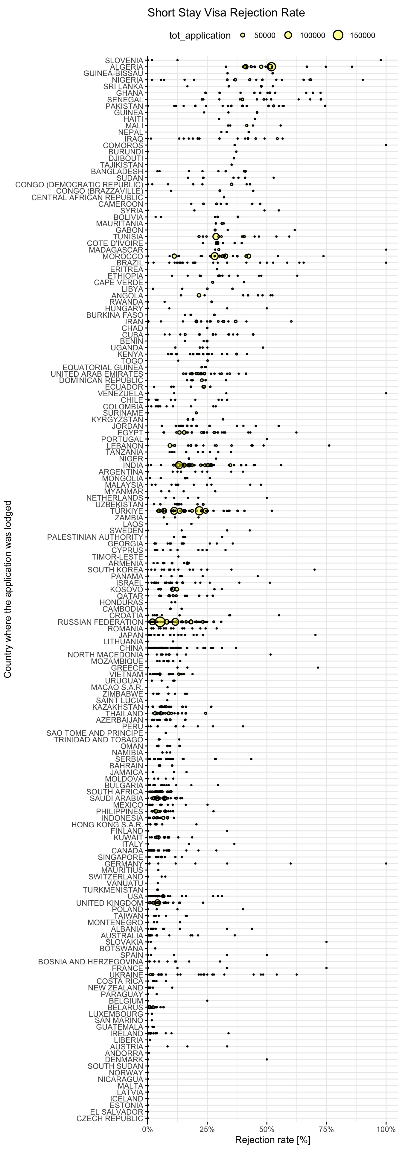
The consulate level is too detailed, let’s try to visualize and then aggregate the data by country where the request was lodged:
country_rank <-
  visa %>%
  group_by(consulate_country) %>%
  summarise(
    mean_rej_rate = weighted.mean(
      x = rej_rate,
      w = tot_application)
  ) %>%
  arrange(mean_rej_rate) %>%
  pull(consulate_country)
visa %>%
filter(tot_application > 0) %>%
ggplot() +
aes(x = rej_rate,
y = consulate_country %>% factor(levels = country_rank)) +
geom_point(
aes(size = tot_application),
shape = 21,
stroke = 1,
fill = '#FFFF0077'
) +
labs(title = 'Short Stay Visa Rejection Rate',
x = 'Rejection rate [%]',
y = 'Country where the application was lodged') +
scale_radius(
range = c(0, 5),
limits = c(1, NA)
) +
scale_x_continuous(
expand = expansion(mult = c(0, .05)),
labels = scales::percent
)
Aggregate by Continent
Let’s try to aggregate the countries by continent, to seek for patterns. We can infer the continent from the string consulate_country with functions from the package countrycode.
visa <-
  visa %>%
  mutate(
    continent = consulate_country %>%
      countrycode(
        origin = 'country.name',
        destination = 'continent'
      )
  )
Warning: There was 1 warning in `mutate()`.
ℹ In argument: `continent = consulate_country %>% countrycode(origin =
"country.name", destination = "continent")`.
Caused by warning:
! Some values were not matched unambiguously: KOSOVOvisa %>%
glimpse()Rows: 1,766
Columns: 8
$ schengen_state <chr> "Austria", "Austria", "Austria", "Austria", "Austria…
$ consulate_country <chr> "ALBANIA", "ALGERIA", "ARGENTINA", "AUSTRALIA", "AZE…
$ consulate_city <chr> "TIRANA", "ALGIERS", "BUENOS AIRES", "CANBERRA", "BA…
$ issued <dbl> 81, 1216, 18, 1754, 1755, 1530, 50, 378, 643, 21, 81…
$ not_issued <dbl> 6, 831, 0, 22, 33, 13, 0, 4, 8, 0, 310, 17, 0, 89, 2…
$ tot_application <dbl> 87, 2047, 18, 1776, 1788, 1543, 50, 382, 651, 21, 11…
$ rej_rate <dbl> 0.068965517, 0.405959941, 0.000000000, 0.012387387, …
$ continent <chr> "Europe", "Africa", "Americas", "Oceania", "Asia", "…And let’s map the continent to the colour of the points.
visa %>%
  filter(tot_application > 0) %>%
  ggplot() +
  aes(x = rej_rate,
      y = consulate_country %>% factor(levels = country_rank),
      colour = continent) +
  geom_point(
    aes(size = tot_application),
    alpha = .9
  ) +
  labs(title = 'Short Stay Visa Rejection Rate',
       x = 'Rejection rate [%]',
       y = 'Country where the application was lodged') +
  scale_radius(
    range = c(0, 5),
    limits = c(1, NA)
  ) +
  scale_x_continuous(
    expand = expansion(mult = c(0, .05)),
    label = scales::percent
  ) +
  scale_color_paletteer_d(
    "awtools::mpalette"
  )
Warning: Removed 9 rows containing missing values (`geom_point()`).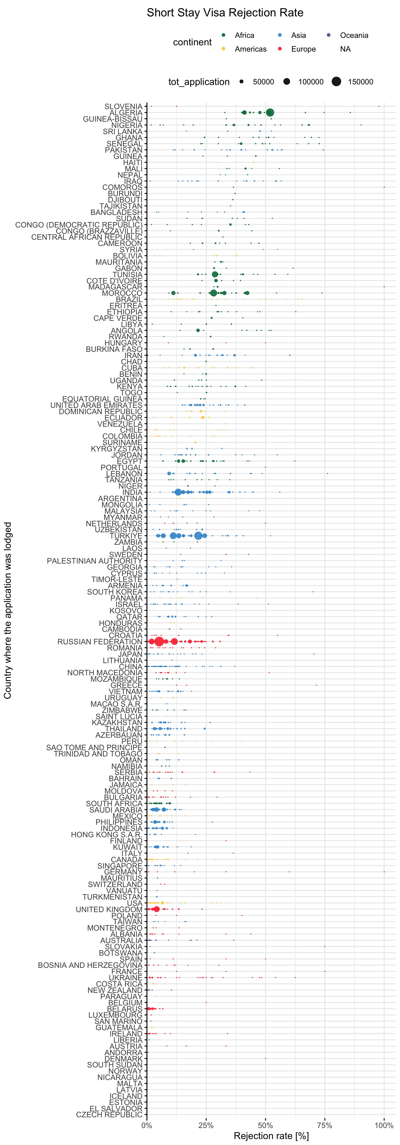
visa %>%
  filter(tot_application > 0) %>%
  ggplot() +
  aes(x = rej_rate,
      weight = tot_application,
      fill = continent) +
  geom_histogram() +
  geom_hline(yintercept = 0) +
  facet_wrap(facets = 'continent',
             ncol = 1) +
  labs(title = 'Short Stay Visa Rejection Rate',
       x = 'Rejection rate [%]',
       y = 'Application Lodged [n]') +
  scale_fill_paletteer_d(
    "awtools::mpalette"
  ) +
  scale_x_continuous(
    expand = expansion(mult = c(0, .05)),
    label = scales::percent
  )
`stat_bin()` using `bins = 30`. Pick better value with `binwidth`.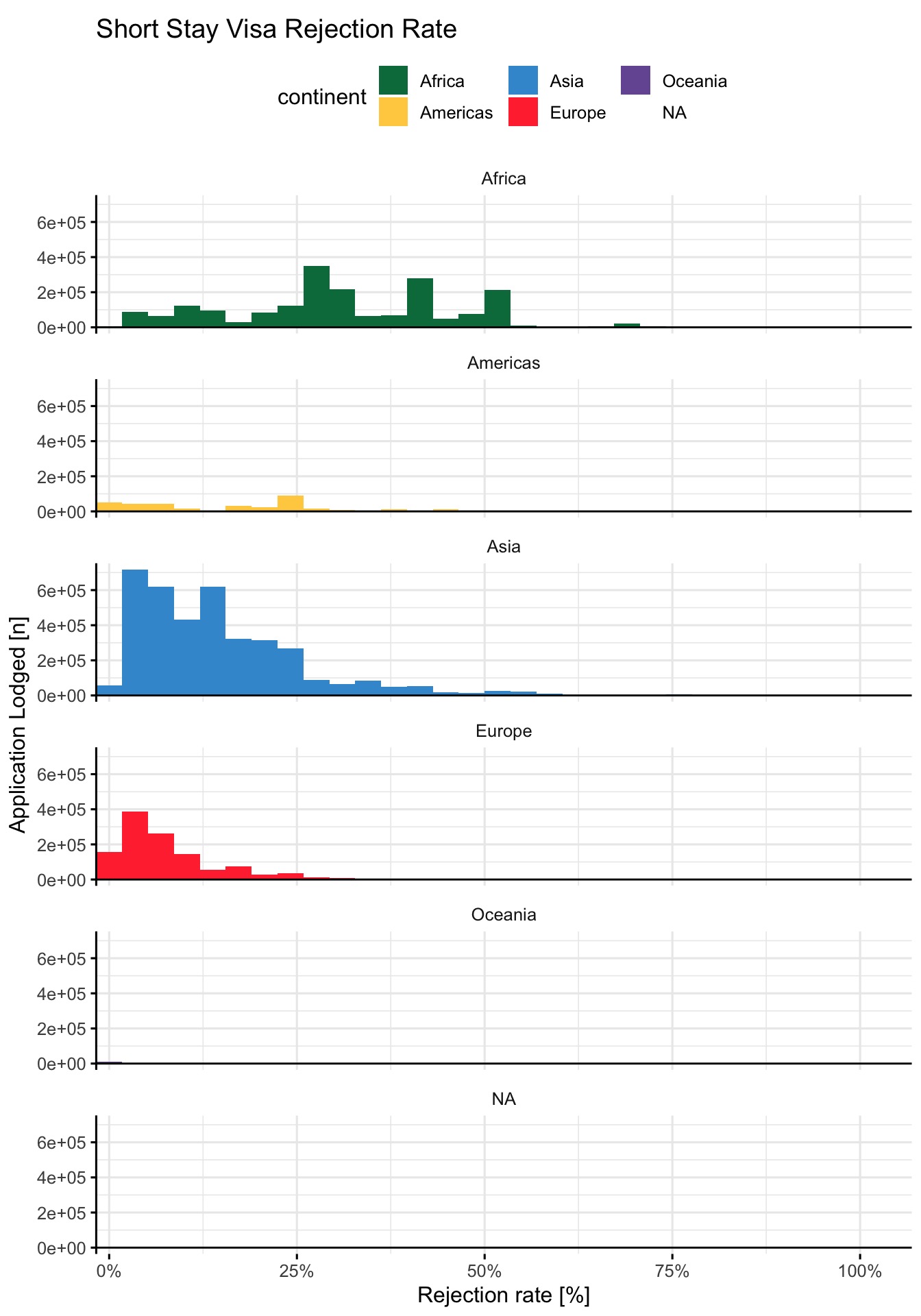
Conclusions
Countries in the African continent face an unexpectedly high rejection rate for Schengen short stay visa applications.
This explorative analysis does not in any way explore the causes of this patterns, but highlights a potential problem that from here on can be described and studied more deeply.